Reproduction and Beyond GSoC (GSoC '23, 4)

To finish off my GSoC experience, Hugo, Orion, and I agreed to start a reproduction of tried and tested transport property calculations in the literature to validate my implementations of self-diffusivity and viscosity. I successfully calculated a self-diffusivity of $2.47 \times 10^-9$ $m^2 / s$ using my Green-Kubo self-diffusivity implementation from a $20$ $ps$ simulation of the SPC/E water model, which agrees well with the results obtained by Kumar, Sarkar, and Bagchi in 2019 as well as Mark and Nilsson in 2001.¹^,² This was a challenging and time consuming process, but it also helped me see the package from a user’s perspective and improved my understanding of running molecular dynamics simulations with a new MD engine. What I find particularly exciting about creating this new package is how it will develop beyond GSoC. I plan to continue the reproduction process with viscosity and implement the Green-Kubo viscosity utility function and my mentors both intend to make their own contributions to the package. I look forward to releasing the package officially and seeing the community make use of it and contribute to making it a better resource for everyone.

Making Plotting Labels Customizable

One of the great benefits of testing a package with a real use case is being able to more easily identify areas for improvement that you may not see while writing code and simple test cases. In my case, I had not thought to make labels customizable until I used OpenMM, which does not natively support file formats containing all the data needed for these calculations. Consequently, OpenMM users must write out velocities in a separate file like velocities.txt and load the velocities into a Universe manually, which prevents MDAnalysis from standardizing the units. This makes custom labels necessary because we want our plots to have the correct units on their labels. After adding this in PR #33, I was then able to specify that velocities from OpenMM used nanometres instead of angstroms in my plots.

The Challenges of Working with a New MD Engine

When Hugo walked me through how to get started with OpenMM, I thought the reproduction would be easy. Once again, I severely underestimated all the potential pitfalls of software development and science and working between different forms of information. Running simulations was easy, but working with velocities was far from straightforward. To obtain velocity information from a simulation in OpenMM, the user must write their own velocity reporter class and write out the velocities in a separate file. Additionally, I wasted a few runs and a lot of hours trying to run a single simulation that would cover all my bases for self-diffusivity and viscosity. In hindsight, this was a naive thought.

If I were to do this again, I would choose an MD engine that natively writes velocities to the same output file like AMBER or GROMACS. I will likely opt for one of the two when I proceed with the Einstein-Helfand reproduction.

Heeding the Literature

Within reason given my time constraints, I followed the best practices paper by Maginn et al.³ I ran a $20$ $ps$ simulation of the SPC/E water model using OpenMM and openmmtools with 1371 water molecules, outputting velocities every 4 fs. While working out this setup, I realized that it was far better to tailor my simulation to one task, calculating self-diffusivity in my case, than to try to cover a lot of ground with a long and costly simulation. It is difficult to run a single simulation in a way that is best for all of a user’s needs and running multiple simulations is good practice.

For reference, I have added my OpenMM script below. If this simulation were to be conducted for real research, I would highly recommend sampling from the correct ensemble as directed in the Maginn et al. paper and running multiple replicates.³

  
from openmm.app import *
from openmm import *
from openmm.unit import *
from sys import stdout

from simtk import openmm, unit
from openmmtools import testsystems


class VelocitiesReporter(object):
    def __init__(self, file, reportInterval):
        self._out = open(file, 'w')
        self._reportInterval = reportInterval

    def __del__(self):
        self._out.close()

    def describeNextReport(self, simulation):
        steps = self._reportInterval - simulation.currentStep%self._reportInterval
        return (steps, False, True, False, False, None)

    def report(self, simulation, state):
        vels = state.getVelocities().value_in_unit(nanometer/picosecond)
        for v in vels:
            self._out.write('%g %g %g\n' % (v[0], v[1], v[2]))


NSTEP = 10000

water_box = testsystems.WaterBox(box_edge=3.5*unit.nanometer, model='spce')
system = water_box.system  # An OpenMM System object.
positions = water_box.positions  # Initial coordinates for the system with associated units.

integrator = LangevinMiddleIntegrator(298*kelvin, 1/picosecond, 0.002*picoseconds)
simulation = Simulation(water_box.topology, system, integrator)
simulation.context.setPositions(water_box.positions)
simulation.minimizeEnergy()
simulation.reporters.append(PDBReporter('wb_output.pdb', 1000))
simulation.reporters.append(DCDReporter('wb_output.dcd', 2))
simulation.reporters.append(VelocitiesReporter('velocities.txt', 2))
simulation.reporters.append(StateDataReporter(stdout, 2, step=True, potentialEnergy=True, temperature=True, remainingTime=True, totalSteps=NSTEP))
simulation.step(NSTEP) # runs 10000 steps

Self-Diffusivity Calculation and Plots

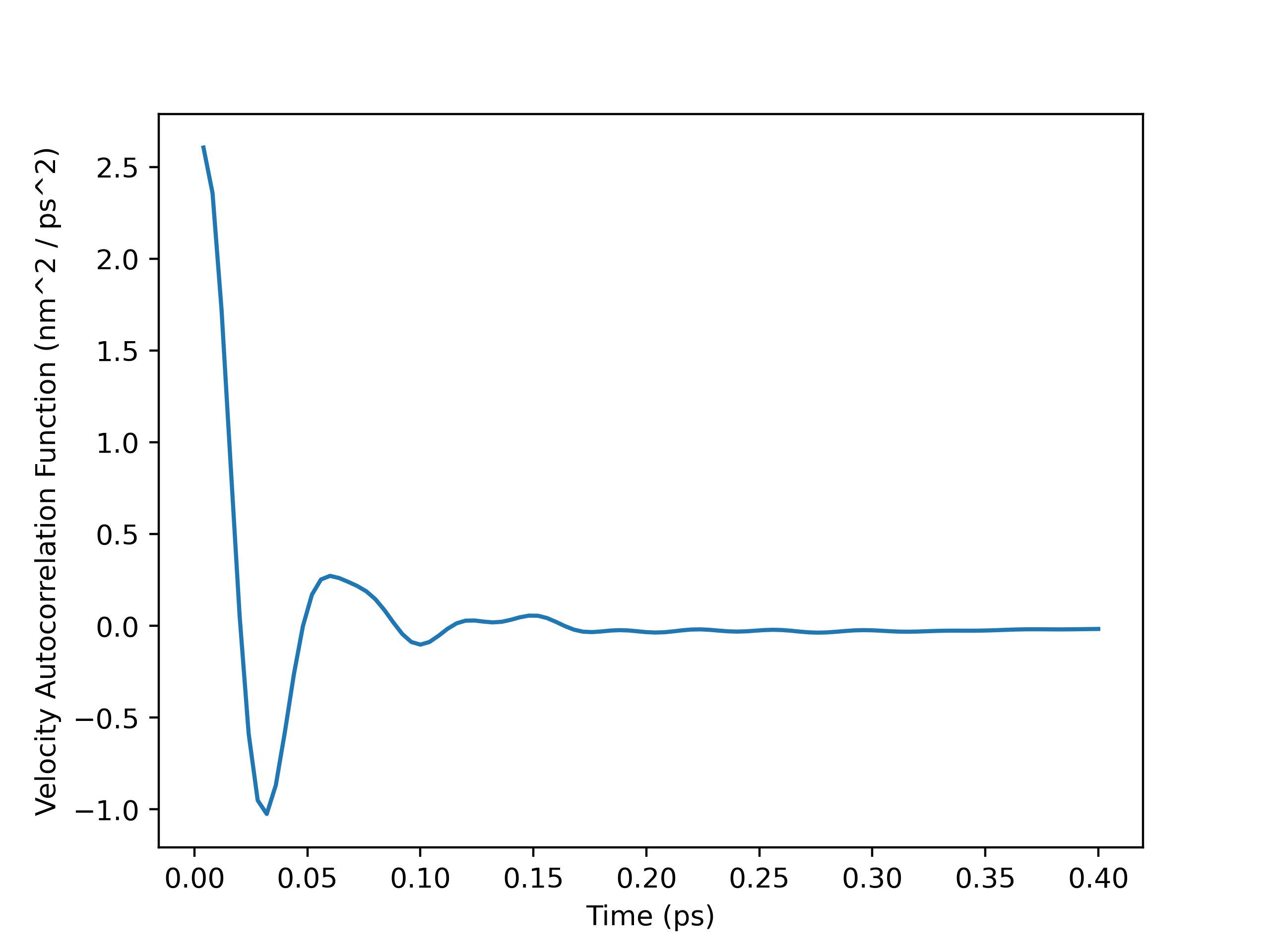
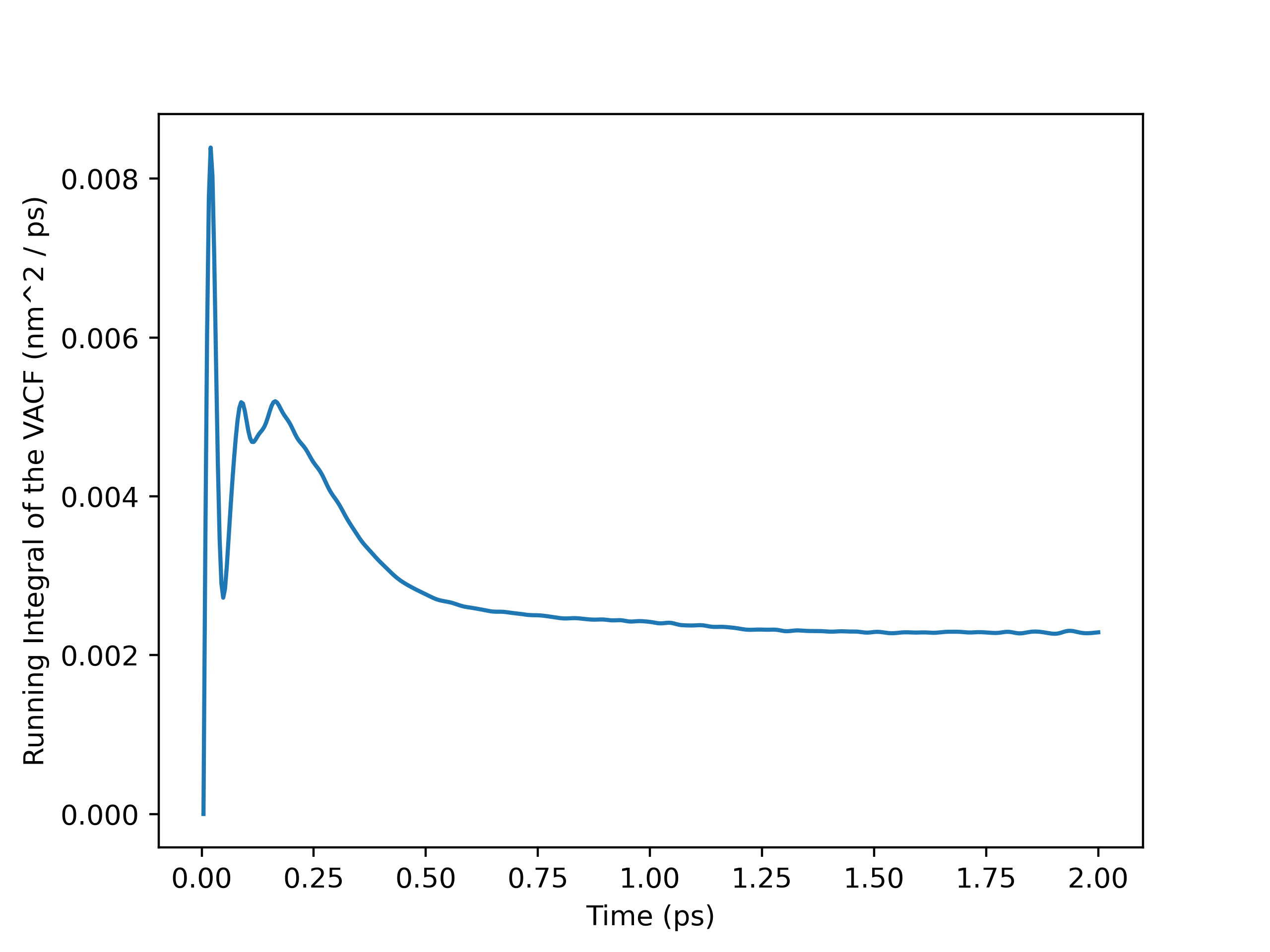
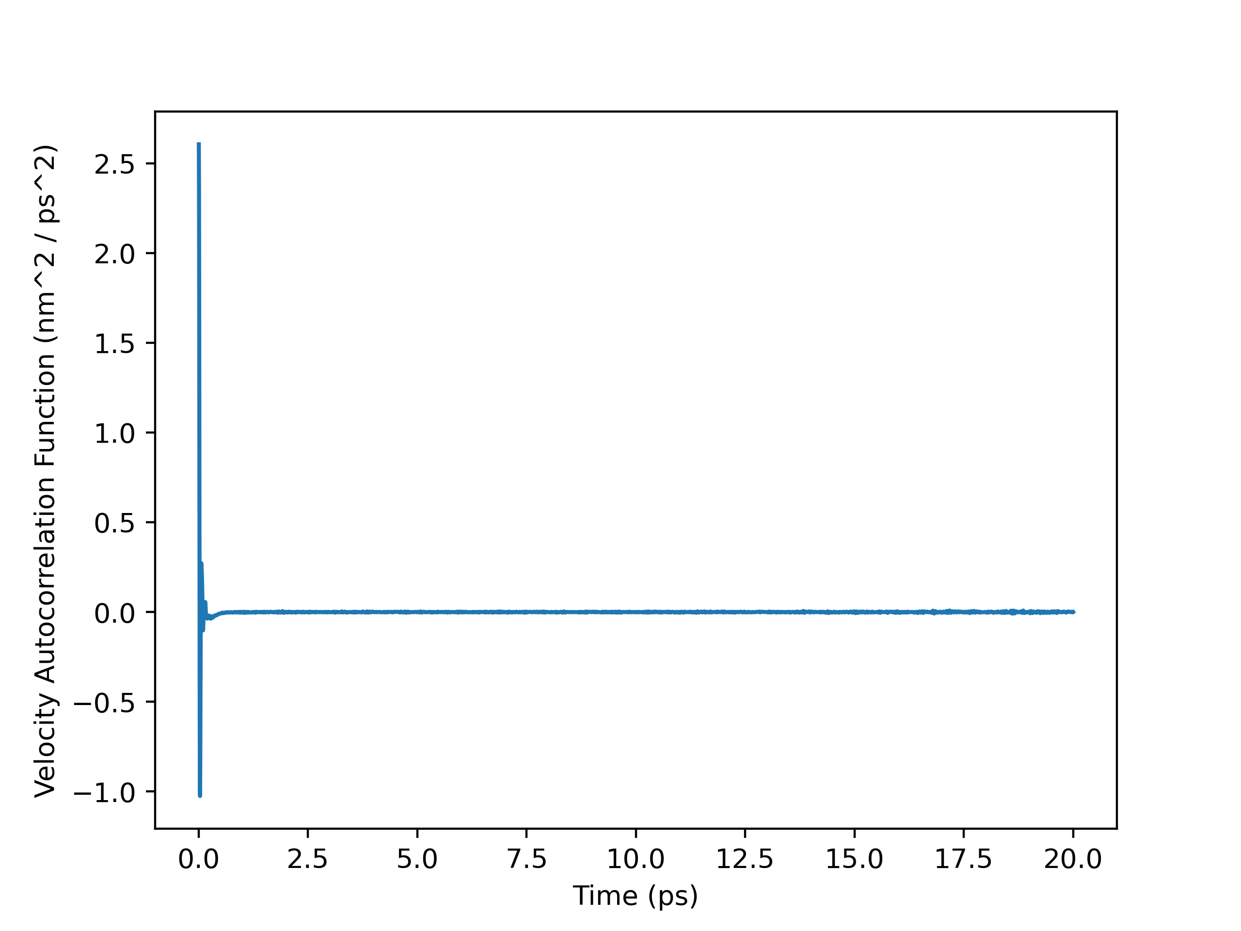
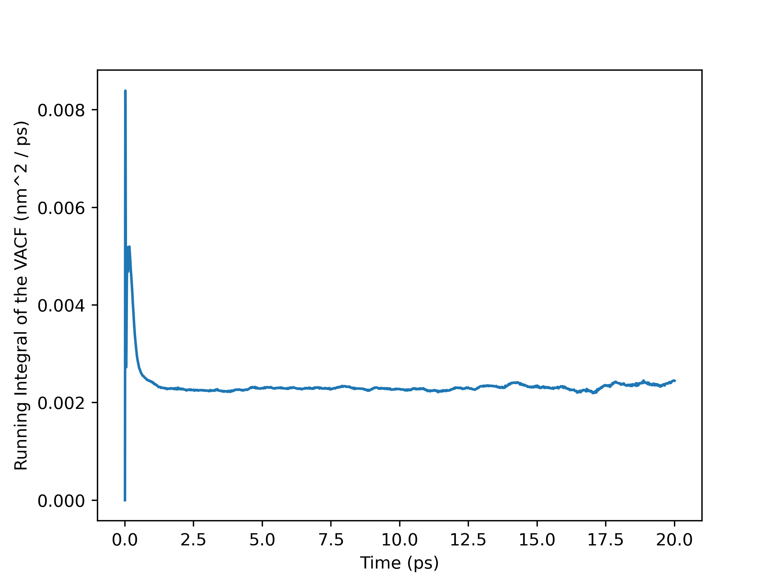
To perform the self-diffusivity calculation with OpenMM-outputted velocities, I had to load the velocities into an MDAnalysis Universe manually with numpy.loadtxt(). I then ran the atoms in the Universe through my VelocityAutocorr class and plotted the velocity autocorrelation function (VACF) and the running integral. From the plots, I decided to calculate the self-diffusivity with a cut-off time of $0.8$ $ps$. My self_diffusivity_gk() method within the VelocityAutocorr class gave a value of $0.002465649307854674$, which is $2.47 \times 10^-9$ $m^2 / s$ in SI units. This result was fairly insensitive to the cut-off time, as self-diffusivity estimates computed after $0.8$ $ps$ were between $2.2-2.5 \times 10^-9$ $m^2 / s$. It is in good agreement with the value of $2.58 \times 10^-9$ $m^2 / s$ obtained by Kumar, Sarkar, and Bagchi and the range of $2.7-3.0 \times 10^-9$ $m^2 / s$ from Mark and Nilsson.¹^,²

VACF Plot

Running Integral Plot

VACF Plot (Full Trajectory)

Running Integral Plot (Full Trajectory)

Lessons Learned

Always plan to spend a lot more time than you expect, both with software development and with science
Having a call with someone more experienced, like Hugo, when starting something completely new can really streamline the learning process
Approaching your software with a real use case from the perspective of a user is a wonderful way to find new areas for improvement
Reading and re-reading papers carefully can save time that would otherwise be spent on unnecessary simulations

Beyond GSoC

The following is simply a list of my own ideas for what we could add to this package and far from exhaustive. We encourage new ideas, GitHub issues, bug reports, and contributions! I intend to continue looking into the Einstein-Helfand viscosity reproduction and complete the Green-Kubo viscosity utility function, but the rest will depend on my availability:

Implement a utility function to calculate viscosity via the Green-Kubo method (planned)
Reproduce literature results using the implemented Einstein-Helfand viscosity class (will continue looking into in consultation with MDAnalysis community)
Implement additional transport property analyses (ionic and thermal conductivity, etc) and tools (utility functions, plotting functions, etc)
Add example Jupyter Notebooks
Continue improving the documentation

References

Kumar, S.; Sarkar, S.; Bagchi, B. Anomalous Viscoelastic Response of Water-Dimethyl Sulfoxide Solution and a Molecular Explanation of Non-Monotonic Composition Dependence of Viscosity. J. Chem. Phys. 2019, 151 (19), 194505. https://doi.org/10.1063/1.5126381. ↩ ↩²
Mark, P.; Nilsson, L. Structure and Dynamics of the TIP3P, SPC, and SPC/E Water Models at 298 K. J. Phys. Chem. A 2001, 105 (43), 9954–9960. https://doi.org/10.1021/jp003020w. ↩ ↩²
Maginn, E. J.; Messerly, R. A.; Carlson, D. J.; Roe, D. R.; Elliot, J. R. Best Practices for Computing Transport Properties 1. Self-Diffusivity and Viscosity from Equilibrium Molecular Dynamics [Article v1.0]. Living J. Comput. Mol. Sci. 2018, 1 (1), 6324–6324. https://doi.org/10.33011/livecoms.1.1.6324. ↩ ↩²