
Contributor: Xu Hong Chen
Mentors: Hugo MacDermott-Opeskin (@hmacdope), Orion Cohen (@orionarcher)
Organization: MDAnalysis
Transport property analyses are among the most requested features in the MDAnalysis project. Biomolecular researchers and chemical engineers routinely use these measurable values describing the transfer of mass, momentum, heat, and charge in their regular work.1, 2 My Google Summer of Code (GSoC) project aimed to add methods for calculating self-diffusivity and viscosity, the two most common transport properties in the literature,1 to MDAnalysis with a focus on user-friendliness and test-driven development. Initially, I proposed to:
- Implement a class to calculate self-diffusivity via the Green-Kubo method
- Write a utility function to calculate shear viscosity via the Einstein method
- Create a utility function to calculate shear viscosity via the Green-Kubo method
- Test and document the new features to ensure they are reliable and easy to use
After some discussion that began with Discord user jenclark’s suggestion to try the Helfand method for viscosity to better integrate the feature wtih MDAnalysis, we shifted our priorities away from the utility functions to focus on a new Einstein-Helfand viscosity class. That extra research and trial and error were well worth the result - better software with a more simple and robust API.
My Summer in Python and NumPy Arrays
My summer culminated in the creation of Transport Analysis, a standalone Python package to compute and analyze transport properties powered by MDAnalysis.
Transport Analysis GitHub: https://github.com/MDAnalysis/transport-analysis
Building a FAIR-compliant Python Package from the MDAKit Cookiecutter Template
Generating my package from the MDAKit cookiecutter template streamlined package creation, ensuring that Transport Analysis was set up through a reliable, stringently reviewed process. The included CI/CD pipeline needed some adjusting on GitHub, but it facilitated writing maintainable software from the very beginning. Pull request (PR) #3 added the new code formatter Black to the CI, while PR #22 flattened the package’s structure to simplify its organization of modules.
Velocity Autocorrelation Functions (VACFs) and Green-Kubo Self-Diffusivity
PR #1 built two implementations of the VACF calculation: a simple “windowed” algorithm and a fast FFT algorithm leveraging tidynamics. All the computations involved are vectorized, but the FFT algorithm speeds the calculations up even further. I designed a simple test system from a unit velocity trajectory and began with some very basic calculations on pen and paper, then gradually wrote more and more tests until my code was tested with the same rigour as the MDAnalysis MSD module on top of reaching 100% code coverage.
PR #23 introduced a plotting method for VACFs via Matplotlib’s object-oriented API, saving users from having to write their own plotting code. PR #24 then makes it easy to calculate the Green-Kubo self-diffusivity with the methods self_diffusivity_gk and self_diffusivity_gk_odd. It also added a new plotting method for the running integral.
Einstein-Helfand Viscosity
PR #25 was challenging because it was not part of the initial plan and the methodology and practices were less prominent in the literature. The calculation itself was also more difficult to work with because it had a lot more terms than self-diffusivity, but I enjoyed the process of learning and developing this class. Like the VACF implementation, it takes full advantage of NumPy arrays and the MDAnalysis AnalysisBase API.
PR #29, which adds plotting functionalities for the Einstein-Helfand viscosity class, is essentially complete but has yet to be merged because we are still considering whether it would be better to leave the plot in standard MDAnalysis units or convert them to SI units. While standard MDAnalysis units are friendly for VACFs and self-diffusivity, that is not the case for viscosity due to the number of terms involved in the calculation. It is the only unmerged PR in the project at the time of writing.
Because we prioritized the new, more user-friendly Einstein-Helfand viscosity class, which turned out to be more time consuming due to the research and complex implementation, I did not get to write the Green-Kubo viscosity utility function within the GSoC timeline. Nonetheless, I am happy to have adapted my original plan to our community discussions and delivered a more useful project. I plan to implement the utility function after GSoC, though I suspect most users will much prefer the Einstein-Helfand viscosity class. Ultimately, I achieved my goals for this summer and I am excited to see Transport Analysis grow as a community resource.
Reproduction of the Literature
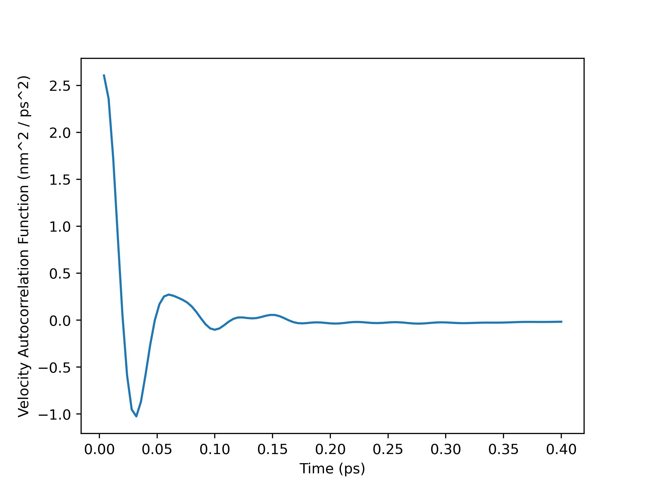
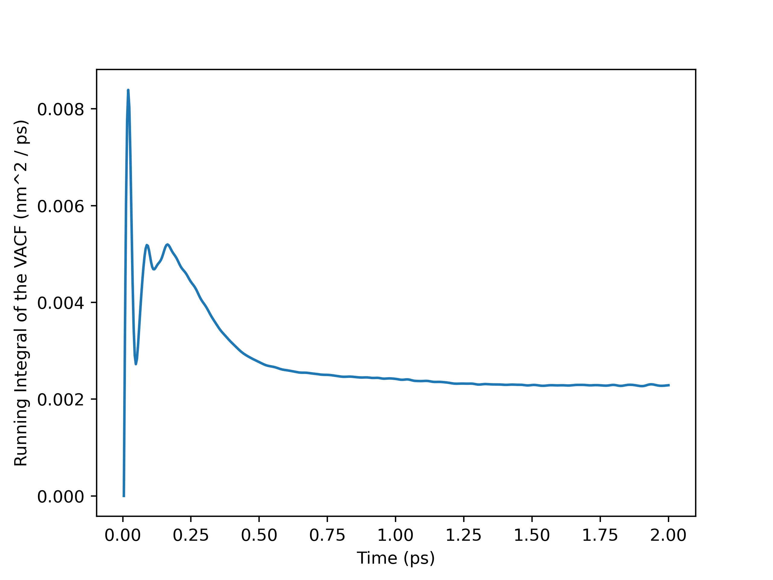
To go beyond testing against simple “toy” systems and test data, I began a reproduction of established transport property calculations in the literature to validate my implementations. I successfully calculated a self-diffusivity of $2.47 \times 10^-9$ $m^2 / s$ using my Green-Kubo self-diffusivity implementation from a $20$ $ps$ simulation of the SPC/E water model at $298$ $K$, which agrees well with the results in the literature.3, 4 A full writeup of this reproduction can be found in my last blog post, Reproduction and Beyond GSoC (GSoC ‘23, 4). Some of the key plots are provided below.
VACF Plot
Running Integral Plot
Using Transport Analysis
Installation
Transport Analysis is nearing release, and it can be cloned and installed from GitHub in a virtual environment. Here is a simple example using mamba.
First, we clone Transport Analysis:
1
git clone https://github.com/MDAnalysis/transport-analysis.git
Then we can go ahead and install the package with mamba and pip. In this case, I have named the environment ta-package:
1
2
3
4
5
6
7
8
9
cd transport-analysis

mamba create -n ta-package

mamba env update --name ta-package --file devtools/conda-envs/test_env.yaml

mamba activate ta-package

pip install -e .
Once Transport Analysis is officially released, this process will be even smoother.
A Quick VACF Example
This example calculates a VACF from a very small set of AMBER test data with velocities. In Python, execute:
1
2
3
4
5
6
# imports
import MDAnalysis as mda
from transport_analysis.velocityautocorr import VelocityAutocorr

# test data for this example
from MDAnalysis.tests.datafiles import PRM_NCBOX, TRJ_NCBOX
We will calculate the VACF of an atom group of all water atoms in residues 1-5. To select these atoms:
1
2
u = mda.Universe(PRM_NCBOX, TRJ_NCBOX)
ag = u.select_atoms("resname WAT and resid 1-5")
We can run the calculation using any variable of choice such as wat_vacf and access our results using wat_vacf.results.timeseries:
1
2
3
4
5
6
7
wat_vacf = VelocityAutocorr(ag).run()
wat_vacf.results.timeseries

# results from wat_vacf.results.timeseries
array([275.62075467, -18.42008255, -23.94383428,  41.41415381,
     -2.3164344 , -35.66393559, -22.66874897,  -3.97575003,
      6.57888933,  -5.29065096])
Notice that this example data is insufficient to provide a well-defined VACF. When working with real data, ensure that the velocities are written frequently enough to obtain a VACF suitable for your needs.
A growing collection of Jupyter Notebook tutorials/examples can be found in the tutorials directory in the repository.
Lessons Learned
Here are a few highlights from my series of blog posts:
- Always check if the dependencies used are up-to-date and/or the expected version
- Look online to see if there are any well-maintained, trustworthy packages as reference for the feature to be implemented (e.g. the MSD module)
- Ask a lot of questions - many of the mentors who were not assigned to my project helped
- Following the GitHub discussions that more experienced developers have can be a fantastic learning opportunity
- Having a call with someone more experienced, like Hugo, when starting something completely new can really streamline the learning process
- Approaching your software with a real use case from the perspective of a user is a wonderful way to find new areas for improvement
The Future
The beauty of open source is the potential for continued improvement and engagement with the community. I will continue working on Transport Analysis after GSoC, and both my mentors intend to make their own contributions to the package. We are always open to new ideas, GitHub issues, bug reports, and contributions. The following is simply a list of a few of the many possibilities for improving this community resource:
- Implement a utility function to calculate viscosity via the Green-Kubo method (planned)
- Reproduce literature results using the implemented Einstein-Helfand viscosity class (will continue looking into in consultation with MDAnalysis community)
- Implement additional transport property analyses (ionic and thermal conductivity, etc) and tools (utility functions, plotting functions, etc)
- Continue adding example Jupyter Notebooks
- Continue improving the documentation
Acknowledgements
I would like to thank MDAnalysis for supporting me from my first PR to my completion of GSoC and beyond. It has been such a wonderful experience discussing software and science on GitHub, Discord, and the mailing lists. I am very grateful for the continued support of my mentors, Hugo MacDermott-Opeskin (@hmacdope) and Orion Cohen (@orionarcher), who have taken the time to have many live calls with me, carefully review my code and the science of my work, and share a wealth of lessons and resources that I will continue learning from well after GSoC.
I would like to extend further thanks to Oliver Beckstein (@orbeckst) for his support throughout my involvement with MDAnalysis and his insights on computational biophysics and programming. I also really appreciated Lily Wang (@lilyminium) and Irfan Alibay’s (@IAlibay) help with setting up the package and the CI. I enjoyed talking about code formatting with Rocco Meli (@RMeli) and I am grateful for Richard Gowers’ (@richardjgowers) reviews of my first analysis class. Finally, I would like to thank Google for offering this program and supporting open-source software.
If any readers are interested in scientific software, molecular simulations, or computational research, I would highly encourage looking into the MDAnalysis community. The developers’ dedication and ability shows in the library’s impressive performance compared to similar software and its unmatched interoperability and support for a wide range of analyses.
References
Maginn, E. J.; Messerly, R. A.; Carlson, D. J.; Roe, D. R.; Elliot, J. R. Best Practices for Computing Transport Properties 1. Self-Diffusivity and Viscosity from Equilibrium Molecular Dynamics [Article v1.0]. Living J. Comput. Mol. Sci. 2018, 1 (1), 6324–6324. https://doi.org/10.33011/livecoms.1.1.6324. ↩ ↩2
Wang, J.; Hou, T. Application of Molecular Dynamics Simulations in Molecular Property Prediction II: Diffusion Coefficient. J. Comput. Chem. 2011, 32 (16), 3505–3519. https://doi.org/10.1002/jcc.21939. ↩
Kumar, S.; Sarkar, S.; Bagchi, B. Anomalous Viscoelastic Response of Water-Dimethyl Sulfoxide Solution and a Molecular Explanation of Non-Monotonic Composition Dependence of Viscosity. J. Chem. Phys. 2019, 151 (19), 194505. https://doi.org/10.1063/1.5126381. ↩
Mark, P.; Nilsson, L. Structure and Dynamics of the TIP3P, SPC, and SPC/E Water Models at 298 K. J. Phys. Chem. A 2001, 105 (43), 9954–9960. https://doi.org/10.1021/jp003020w. ↩